I came across ornata's fly project, which connects a simulated fruit fly network to video games, and wanted to try building something along similar lines in the browser. The part that interested me was being able to follow the whole process: what goes into the network, what happens to the signals, and how those signals become a move in a game.
That became Fly Plays. It uses 166,700 retained neurons and 25,582,938 weighted connections from a real fruit fly wiring map, with Space Invaders and Tetris as the games. Your browser runs the simulation and a small controller that starts without knowing how to play.
There are several different ideas packed into that description. I will try to explain them through examples, since I think following one signal through the system is more useful than just listing the components. I have also included the equations used by the implementation, with the symbols introduced as they appear. You can follow the examples first and return to the equations for the details.
Bear in mind that this is an engineering experiment with simplified models of neural activity. The first comparisons haven't shown consistent improvement at the games. I will get into those results as well, because getting something to run and showing that it learns something useful are separate things to establish.
First, having a map
A connectome is a map of nerve cells and the connections between them. The dataset used here is called MaleCNS, and it covers a male fruit fly's brain and ventral nerve cord. The nerve cord is part of the system involved in controlling the body.
For an engineering analogy, picture a road map. It tells you which places are connected and which paths you could take. If you wanted to simulate traffic, though, you would still need to decide how cars behave, when they enter a road, and how they affect each other.
The map gives you structure. A simulation needs rules for what happens on that structure.
This distinction carries through the whole project. I can use the measured connections to decide where a signal goes, while still making a fairly rough assumption about what that signal does when it arrives.
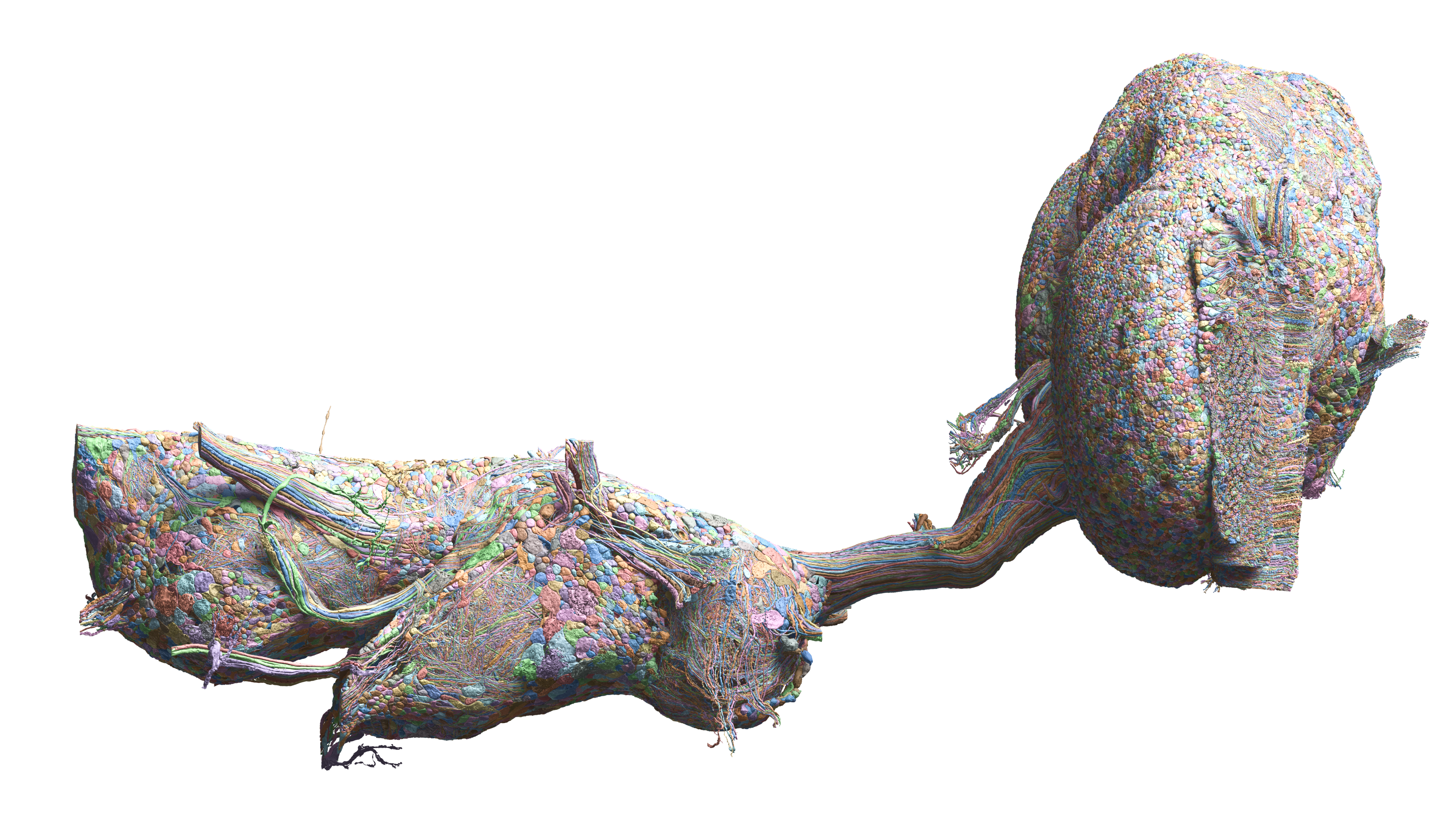
The MaleCNS reconstruction shown in Google Research's article. The large image shows reconstructed anatomy; the flashing dots in Fly Plays show activity calculated by my simulation.
The work behind that map
MaleCNS came from a collaboration led by HHMI Janelia, with Google Research, the University of Cambridge, and the MRC Laboratory of Molecular Biology. The researchers used high-resolution electron microscopy to image the tissue, then reconstructed and checked the cells and their connections. Janelia's account of the project describes how the imaging, computation, proofreading, and cell labeling fit together.
The motivation is to understand how neural circuits produce behavior. Having the brain and nerve cord in one map lets researchers follow paths from sensory input toward the systems controlling movement. It also gives them a way to compare male and female circuitry, including circuits involved in social behavior. Those are the research questions behind the dataset; the arcade is something I added afterward.
Google's part: tracing the cells
Google Research helped turn microscope images into three-dimensional reconstructions of nerve cells using AI. This involves segmentation, which means identifying which parts of an image belong to which object. Human experts then checked and corrected the reconstruction. Google also developed Neuroglancer, a tool for exploring large datasets like these. Google's explanation of the MaleCNS work is a good starting point.
Take for instance a cell with a long, branching extension passing close to another cell. A reconstruction has to follow that extension without accidentally joining it to its neighbor. If it joins them, the resulting wiring map can contain connections that shouldn't be there.
One approach Google developed is the flood-filling network. It starts from a location and repeatedly predicts which surrounding image pixels belong to the same object, growing the region as it goes. You can think of this as following one thread through a tangled pile, using what you've already followed to guide the next step. The real method works on three-dimensional image data. Google's earlier explanation of flood-filling networks includes animations of that process.
This is an example of AI being used to help construct a scientific dataset. Once the map exists, other people can build experiments that use it. The AI doing the image reconstruction and the controller playing a game here have different jobs.
From the research files to something a browser can use
The official release includes cell annotations, neurotransmitter predictions, connection tables, and much larger imaging data. The connection-strength table alone is around 1.1 GB. Loading all the research files and preparing them on every visitor's device would make for a fairly unpleasant first visit, especially on a phone.
I prepare the runtime files ahead of time with a Python script. The process is reproducible, and after the original downloads it can run offline.
First, the script keeps cells with a nonempty broad cell-class annotation, including provisional annotations. It keeps every connection between those retained cells. That produces the same 166,700 cells and 25,582,938 weighted connections documented by the reference project's technical notes.
N.B. those 25.6 million weighted connections and the roughly 125 million synapses reported for MaleCNS count different things. Several synaptic contacts between the same source and destination can contribute to one weighted connection. The browser is working with a graph of connections between retained neurons, rather than a separate simulated object for each anatomical contact.
Each retained cell gets a compact numeric index. The connections are grouped by their source cell, so when cell 42 fires, the engine can go directly to the list of cells it connects to. There is no need to search the entire graph to find its neighbors.
The preparation also assigns positive or negative influence using the source cell's predicted neurotransmitter and normalizes the incoming connection magnitudes for each destination. In this model, GABA, glutamate, and histamine are treated as inhibitory. Other or unknown transmitters are treated as excitatory. This is a coarse modeling choice; the resulting numbers aren't measurements of the exact electrical effect at every synapse.
Writing the connections as a matrix
To make the normalization precise, let be the nonnegative source-data strength of a connection from neuron to neuron . The destination is the first index. Let be +1 or -1 according to the transmitter rule above. The prepared weight is:
The denominator adds the strengths entering neuron . The maximum with one avoids division by zero. For the retained data, the preparation script checks that each nonempty incoming row has absolute weights summing to approximately one.
For example, suppose three inputs have strengths 2, 3, and 5, and only the second input is inhibitory. They become:
Their absolute magnitudes sum to one, but their signed sum is 0.4. If all three source cells fire together, their combined input is therefore 0.4. Excitation and inhibition partly cancel.
Conceptually, these weights form a sparse matrix . Most entries are zero, and the browser stores only the retained connections rather than allocating that enormous dense matrix. Its graph can contain loops, so activity can influence later activity. There is no sequence of conventional feedforward layers here. This matrix stays fixed throughout training.
The output is a set of compact numeric arrays, compressed into 32 runtime chunks. They total about 139 MB, or 132 MiB in the units shown on the page. All retained connections remain in those arrays. I didn't remove weak connections to make the simulation faster.
Now let's follow one game picture
At a high level, the loop looks like this:
Game picture
    ↓
Simulated eye cells
    ↓
Signals through the fly's wiring
    ↓
Recent activity from output cells
    ↓
Controller chooses a button press
    ↓
Game changes and gives feedback
    ↓
Repeat
There are a few choices hidden inside each arrow, so let's go through them.
1. Give the network something to see
The game renders a small grayscale picture of its playfield, 64 pixels wide and 48 pixels tall. This is the picture you see in the vision panel. The score display, buttons, and explanatory text around the game stay out of it.
Imagine an enemy moving across an otherwise dark part of the Space Invaders screen. Some pixels get brighter and others get darker. The simulation uses both brightness and changes from the previous picture to stimulate 6,006 annotated photoreceptors, which are the cells serving as the simulated eyes.
The screen-to-cell mapping uses published information about visual columns where available, connections to assigned cells for others, and deterministic estimates for the remaining cells. It is approximate. A 64 by 48 pixel game screen doesn't suddenly become an accurate model of a fly's optics because I connected it to cells labeled as photoreceptors.
This is one of the first places I would look when trying to improve the experiment. A useful network can still receive a poor representation of the thing it is supposed to respond to.
For the equations, I will use for a neural step and later for a controller decision. They run on different clocks.
Let be the mapped pixel brightness for photoreceptor , divided by 255 so it lies between zero and one. The change in brightness and the resulting stimulation are:
The brightness term responds to a visible object, while the change term responds to either brightening or darkening. If a pixel changes from 0.2 to 0.8, the expression inside the minimum is 1.32, so the input is capped at 0.62. If it remains at 0.8 on the following neural step, the change term is zero and the input is 0.2232.
The game image is refreshed every five neural steps and held between those updates. The previous brightness is updated on every neural step, so a newly observed change contributes once, rather than being counted five times. Other cells receive no direct visual stimulation. These choices encode a picture into activity; they do not identify enemies or good Tetris placements.
2. Pass signals through the wiring
The cells use a model called leaky integrate-and-fire. The name sounds more complicated than the basic idea.
Picture a bucket with a small leak. Incoming activity adds to it, some activity fades over time, and when it reaches a threshold the cell fires and resets. That firing then affects the cells connected to it. Depending on the modeled connection, it can push a neighbor toward firing or pull it away.
For a made-up numerical example, suppose a cell is at 0.7 and its threshold is 1. After some activity fades, it is at 0.6. If the net incoming signal adds 0.5, it reaches 1.1, fires, and resets. If that incoming signal had been negative, it might instead have moved farther from the threshold.
The exact values in that example are just to build intuition. The implemented model has its own decay, gain, background input, and threshold settings. It also includes seeded background activity, so the visual input isn't the only thing capable of making a cell fire.
The engine advances in steps of 20 milliseconds of simulated time. At each step it updates every retained cell, and activity from cells that fired on the previous step travels through their outgoing connections. This lets the engine avoid propagating spikes from cells that didn't fire, while preserving the graph and every scheduled neural update.
Here is that update using the actual constants. Let be one if cell fired on the previous step, and zero otherwise. Its contribution to cell is its spike multiplied by the fixed connection weight. Adding all contributions gives:
This is a sparse matrix-vector multiplication in mathematical terms. The engine computes it by traversing the outgoing connections of cells that fired.
With a 20 ms step and a 100 ms decay time constant, the amount of old voltage retained is:
Write for the previous voltage and for the new voltage before checking the threshold:
The 1.5 multiplies the connection input. The 0.18 is constant background drive. The random background contribution is 0.22 with probability per cell per step, and zero otherwise. It is generated by a seeded pseudorandom sequence. Voltages here are model units, not measurements in millivolts.
The threshold and reset complete the update:
The indicator in the first equation returns one when its condition is true. The second equation sets the voltage to zero after a spike and otherwise keeps the updated value. Initially, voltages and spikes are zero.
For a worked step, take a previous voltage of 0.7 and net connection input of 0.2, with no visual input or random impulse on that step:
The cell fires, resets, and influences its neighbors on the next step. This one-step delay means a signal does not traverse the entire graph instantly.
There is temporary memory in the remaining voltages and circulating activity. That is different from learning: the state changes on every step, while the connection weights do not. The equations summarize the implemented recurrence; they are not a detailed biophysical model of a living cell.
The brain panel shows 4,096 sampled cells at measured positions, projected into two dimensions. Their brightness follows simulated firing with a short fade. The other cells are still running; they just aren't all being drawn.
3. Turn activity into a move
The controller reads recent firing activity from 1,316 descending neurons, cells that carry signals away from the brain. These rates summarize a short window of activity rather than just whether a cell fired at one instant.
Ten times per simulated second, the controller produces probabilities for the available actions. In Space Invaders, those include waiting, moving, firing, and moving while firing. In Tetris, they include moving, rotating, dropping, and waiting.
For example, suppose the controller gives moving left a 40% chance and firing a 20% chance. Moving left is more likely, but the controller can still pick another action. Trying different actions is part of the learning process. The action bars on the page show those probabilities.
The controller's inputs are these neural rates and a bias term, which lets it develop a general preference for an action. It doesn't get the enemy coordinates, a list of occupied squares, or a description saying that a Tetris piece would fit nicely in the gap on the right.
That restriction matters to the question I want to explore. Any useful information about the playfield has to reach the action chooser through the simulated neural activity.
From spikes to controller inputs
For each descending neuron, the engine counts spikes over the last 13 neural steps, or up to 260 ms. During startup, it uses only the steps available. With neural steps numbered from one:
This is a firing fraction, not directly a rate in hertz. Four spikes in a full window give . Dividing by the 0.02-second step would express it as a rate of about 15.4 Hz.
At each decision, the learner scales and clips those 1,316 fractions, appends a bias, then normalizes the complete vector. Let mean the fraction available at decision :
The norm is the square root of the sum of squared entries. Appending one makes it nonzero even when all readout neurons are silent. The bias is normalized too, so its final value is not always one.
Scaling and clipping limit how large an individual firing feature can become; normalization controls the overall input scale. They also discard information. For instance, firing fractions of 0.3 and 0.8 both become one before normalization. That may matter if their difference would help choose an action.
Six action scores and one value estimate
Each game has six actions. The actor holds one vector of 1,317 weights for each action, written . It computes an action score, or logit, with a dot product:
A dot product multiplies corresponding entries and adds them. A positive weight makes the associated feature support that action; a negative weight pushes the other way. The actor then applies softmax:
Here . Subtracting the largest score preserves the probabilities while avoiding unnecessarily large exponentials. This is the same logits-to-probabilities operation used in language-model sampling, except the choices here are game actions rather than vocabulary tokens.
The browser samples an action from these probabilities. It can choose a lower-probability action, which gives it opportunities to explore. The actor starts with seeded random weights between -0.01 and 0.01.
The critic has a separate vector , initially zero, and predicts a value:
This lowercase contains trainable critic weights; it is separate from the fixed connectome matrix . The value estimates discounted future reward under the current policy. It is not the game score, a probability of winning, or an oracle that already knows the right action.
The parameter count per game is:
That is 7,902 actor parameters and 1,317 critic parameters. Each game has its own controller. The 25.6 million connectome weights are not included because none of them are trained.
What learning from scratch means here
The controller starts with small seeded random weights, without a policy already trained to play either game. Its decisions can then change as it gets feedback.
The method is called actor–critic. The actor chooses actions. The critic estimates how much future reward might follow from the current input. After a move, the learner compares the reward and its next estimate with what it expected before.
If the outcome is better than expected, the update generally makes the chosen action more likely for similar input. If it is worse, the update pushes in the other direction. The critic adjusts its estimate too. The implementation also encourages some exploration and bounds its updates, so a large reward doesn't produce an arbitrarily large change.
Take the earlier example of moving left and firing. If an enemy gets hit later, the learner receives a positive reward. But it still has to work out whether the earlier activity and action were useful predictors of that outcome. A single reward doesn't explain the rules of Space Invaders to it.
This gets harder when a useful action only pays off much later. In Tetris, placing one piece well may help you clear a line several pieces from now. Deciding which earlier choices deserve credit is a real part of the problem.
The fly network's connections stay fixed during all of this. The small readout controller is what learns. Reloading with a saved checkpoint also means the controller is continuing its practice; it only starts from scratch on a fresh browser or after Reset learning.
The error that drives an update
Suppose decision uses input and selects action . The game applies that action over the following neural steps. Let be the accumulated reward until the next decision, or until the episode ends.
The controller normally updates every five neural steps, or every 0.1 simulated seconds. It first learns from the preceding action, then chooses the next one. There is no preceding action to learn from at the first decision. A terminal transition is learned immediately, even if it occurs before the next scheduled decision.
Let be one when the episode ends and zero otherwise. The critic's target and temporal-difference error are:
At a terminal transition the future-value term is omitted entirely. The 0.99 is the discount factor per controller transition: future rewards contribute slightly less than immediate ones. Both value estimates use the critic weights before the update.
For example, suppose the critic expected 2.0, the observed reward is 1.0, and it estimates 2.5 from the next input:
The outcome was better than expected. If the old estimate had instead been 4.0, the same positive reward would produce an error of -0.525. A positive reward alone does not determine the direction of learning. The comparison with the prior expectation matters.
Updating the critic and actor
The implementation bounds both the error and the weights. Define clipping as:
The error actually used is . For each critic input coordinate , the update is:
The 0.05 is the critic learning rate. Ignoring clipping, this is a step that reduces squared prediction error while treating the target as fixed. That treatment is called a semi-gradient update: it does not differentiate through the next-state value in the target.
For the actor, first consider the reward-driven part of the update. The softmax log-probability gradient gives:
The indicator is one for the selected action and zero for the other five. If the error is positive, the selected action receives a positive coefficient and the alternatives receive negative coefficients. Multiplying by the old input vector makes the change depend on the features present when that action was chosen.
The learner also includes an entropy term to discourage prematurely concentrating all probability on one action. To match the numerical guard in the implementation, define:
Entropy is larger for a spread-out distribution and smaller when one action dominates. The complete coefficient and actor update are:
Here 0.015 is the actor learning rate and 0.01 controls the entropy contribution. The probabilities and features are those saved when the preceding action was selected, not recomputed after changing the weights. The logarithm guard, error clipping, and weight bounds are implementation safeguards, not biological mechanisms.
As a small example, suppose the chosen action had probability 0.2, an input coordinate was 0.5, and the clipped error was 1.475. Ignoring entropy and weight clipping, that action's weight for this coordinate increases by:
This illustrates one coordinate of one update, not a measured improvement in game performance. Repeating such updates changes the action distribution for inputs with similar features.
The connection to machine learning
The actor is mathematically similar to a softmax classifier, but there is no training label saying which move was correct. In supervised learning I could supply an image and a target action. Here the controller must act, receive feedback, and estimate which choices improve future reward. That makes this reinforcement learning.
The critic is a regression model whose targets partly come from its own next-step predictions. The actor uses the resulting error as an estimate of whether its sampled action was better or worse than expected. This combination is a simple online actor-critic method.
The fixed recurrent network serves as a feature extractor with temporary memory. This is a reservoir-style architecture: a changing internal state feeds a trainable readout, while the internal connections stay fixed. Calling it reservoir-style describes the arrangement; it does not establish that this particular wiring and these dynamics produce useful features.
There is no backpropagation through the fly network, no learned retinal mapping, no replay buffer, and no eligibility trace that explicitly carries an update back across a sequence of earlier actions. Delayed rewards must influence earlier decisions indirectly through value estimates over repeated experience. If different situations produce nearly the same readout, a linear controller may have little basis for choosing different moves.
For more background, Sutton and Barto's Reinforcement Learning: An Introduction develops temporal-difference learning and actor-critic methods. The equations here describe this implementation, including its simplifications and numerical bounds.
Giving feedback in each game
Space Invaders has relatively frequent events to reward. Destroying an enemy gives +1, completing a wave gives +3, and losing a life gives -5. The game includes waves, shields, shooting, and three lives.
Tetris uses a 10 by 20 board and a seven-piece bag, so each set of seven pieces contains each shape once in a shuffled order. It supports rotation, soft and hard drops, line clearing, and increasing gravity.
Clearing one, two, three, or four lines gives rewards of 1, 3, 5, or 8. Reaching the top gives -5. I also added smaller feedback based on changes in stack height and holes, bounded to keep those hints from growing arbitrarily large.
This is called reward shaping. You are giving the learner intermediate hints about progress toward the task.
Counterpoint: those hints reflect my assumptions about what is useful. Keeping a stack low is generally helpful, but a move that temporarily makes the stack taller could be part of a better plan. A reward function can encourage behavior that looks good by its own numbers while missing the thing you actually care about.
The game code can inspect the board to calculate a reward. The action chooser receives the resulting number, along with neural activity. Board features aren't secretly being passed in as extra instructions for its next move.
The Tetris shaping term
The exact board heuristic uses the sum of the ten column heights, not just the tallest column. Let be the settled board, the height of column , and the number of empty cells beneath an occupied cell in their column:
After a piece locks and completed lines are removed, the shaping contribution is:
For example, increasing the total column height by four and adding one hole contributes -0.27. Reducing height or removing holes can contribute a positive value.
The line-clear reward and any game-over penalty are added separately. A piece that locks above the board ends the game with -5 immediately. Although this heuristic is written using a board potential, the clipped difference is not the usual discounted potential-based shaping construction. I am not assuming it preserves the optimal policy of a game rewarded only for clearing lines. It changes the learning objective, which is another reason to evaluate actual cleared lines separately from reward and displayed score.
Did it actually improve?
The first evaluation was deliberately small: three training episodes, each capped at 90 simulated seconds. I then froze the trained controller and compared it with an untrained frozen controller and random actions across three fixed evaluation seeds. Each evaluation episode was capped at 45 simulated seconds.
Freezing the trained controller makes it easier to compare the behavior it learned without continuing to change it during the comparison. The same evaluation seeds make the starting conditions more comparable, although different actions can still lead to very different games.
These are the mean game scores, rounded to one decimal place:
| Game | Trained, then frozen | Untrained, frozen | Random actions |
|---|---|---|---|
| Space Invaders | 1,103.3 | 1,066.7 | 1,163.3 |
| Tetris | 242.7 | 267.0 | 238.3 |
The trained Space Invaders controller slightly exceeded the untrained one, but random actions scored higher than both. The Tetris results also didn't show a consistent advantage from training. None of the compared controllers cleared a Tetris line.
N.B. Tetris awards game score for dropping pieces as well. A positive score can therefore look encouraging even when the controller hasn't achieved the central task of clearing lines. Game score and the reward used for training aren't the same number. Looking at cleared lines changes how you interpret that result.
Three seeds and a few short training episodes are a small test. They don't establish long-term improvement or prove that improvement is impossible. They tell me that I haven't demonstrated reliable game learning with this setup yet.
I also checked that changing the visual input path changes downstream readout activity. In a 100-step comparison, connected and disconnected visual input produced different readouts on 90 steps. That shows the input has a causal effect in this model. It doesn't establish that the resulting activity contains a useful strategy for playing the game.
I think it's useful to keep those claims separate. The input affects the network, the learning rule updates the controller, and the games run. Whether the entire combination reliably learns to play better still needs more evidence.
Fitting it into a browser
There is a practical engineering problem here as well: running a large simulation without making the page stop responding.
The network, game state, and learner live together in one Web Worker. Think of it as a separate worker handling the experiment while the main browser thread deals with the page and draws the pictures. The worker sends small snapshots containing things like the game pixels, sampled activity, action probabilities, and scores. It doesn't keep copying the whole network back and forth.
The main loop works in bounded batches. If your device can't keep up, simulated time slows for both the game and the network. At 0.5× actual speed, one second in the simulation takes about two seconds on your clock. This preserves the sequence of neural updates instead of skipping parts of the simulation to match real time.
In the desktop browser checks on my M2 machine, a fresh load ran at roughly 1× simulation speed with 30 frames per second. The reconstructed graph arrays alone occupy about 196 MiB, before the rest of the application and browser overhead. I also tried it on my iPhone 17 Pro Max, where it ran smoothly without any issues during my testing. That's a hands-on observation rather than a measured mobile benchmark; I haven't tested other phones or Android devices.
Each game has its own controller and saved progress. The browser periodically writes the learned weights, counters, and recent scores to IndexedDB, its local database. Switching games starts a new round for that game while preserving its practice. Restart also preserves practice. Reset learning clears the selected game's progress.
If browser storage is unavailable or full, it can keep running for the session, with a notice explaining what won't persist. Switching away from the page pauses the experiment. Nothing about the saved learning syncs across devices.
The download is its own problem
The simulation happens on your device, but the initial wiring still has to get there. I host the prepared chunks on Cloudflare Pages, with the existing Vercel copy as a backup. The browser requests the files directly from Cloudflare, so the large download normally bypasses the site's Vercel bandwidth allowance.
Every chunk is checked against its expected size and SHA-256 checksum before use. Think of the checksum as a way to check that the bytes received match the prepared file. Completed chunks are cached locally when possible, and retries reuse them.
If the primary host fails, returns a damaged file, or stops sending data for 15 seconds, the loader switches to Vercel for the rest of that load. The cached files use the same keys whichever host supplied them. Moving hosting therefore doesn't force a returning visitor to download everything again.
This is a fairly ordinary piece of engineering, but it matters to whether someone can actually try the interesting part of the project.
Where I want to take it next
The next useful work is to run longer comparisons across more seeds and change one modeling choice at a time. I would start with the visual mapping, the activity reaching the readout, and the reward setup. It would also be useful to compare the measured wiring with controlled alternatives to see whether its particular structure contributes anything to game performance.
Adding more games is tempting, but understanding why the current setup does or doesn't improve would teach me more than another game tab by itself.
In So you want to learn AI, I wrote about continuing to build as you learn and paying attention to the limits of your tools. This project is an opportunity to do that. It brings together data preparation, simulation, reinforcement learning, and browser engineering, and gives me a concrete result to question at each stage.
You can try Fly Plays here. Watch the vision panel, the cell activity, and the action probabilities together. Give it a few rounds, then compare the scores. The point is to make the process visible enough that you can start asking which part is doing something useful, and which part still needs work.
The underlying MaleCNS data is credited to FlyEM / HHMI Janelia, Cambridge, MRC LMB, and Google Research under CC BY 4.0. My version modifies its indexing, weights, visual mapping, and packaging for this experiment. ornata/fly provided the inspiration; the browser engine and games are independently implemented in TypeScript.